ML Code 01 - mnist keras
Code Info
- Date:
- Lecturer: Giorgio Gambosi
- Code: ./ml_01_mnist_keras.py
In this code example we have seen how to train a neural net using
the mnist dataset in order to automatically classify handwritten
digits.
1 Imports
As far as the imports go, we have the usual python libraries such as
pandas, numpy and matplotlib. We also have scipy and more
importantly the deep learning library keras.
To actually import all this stuff the following requirements have to be met through pip, the dependency manager of python.
pip3 install pandas
pip3 install matplotlib
pip3 install sklearn
pip3 install keras
pip3 install tensorflow

# these are arch-linux specific package managers
sudo pacman -S cuda
yay -S cudnn
Then imports are then the following ones
import pandas as pd
import numpy as np
import matplotlib.pyplot as plt

from pylab import subplot, imshow, title, gray, NullLocator

import scipy.misc as mi
import scipy.special as sp

from PIL import Image
from itertools import chain
from sklearn.metrics import confusion_matrix, accuracy_score, precision_recall_fscore_support

from keras.datasets import mnist
from keras.models import Sequential
from keras.layers.core import Dense, Dropout, Activation
from keras.utils import np_utils
from keras.models import model_from_json

from keras.layers import Flatten
from keras.layers.convolutional import Conv2D
from keras.layers.convolutional import MaxPooling2D
from keras.utils import np_utils
from keras import backend as K
2 Functions
To deal with this code example the following functions have been defined.
2.1 Plotting of Data
2.1.1 displayData()
The function displayDat() is used to plot elements of the dataset, which in our case are matrices which represents digits.
def displayData(X, t, rows=10, cols=10, img_ind=None, size=16, class_value=False):
    if len(X) > rows * cols:
        # -- get random permutation of rows*cols indices representing
        # -- values in X.
        img_ind = np.random.permutation(len(X))[0:rows * cols]
    else:
        img_ind = range(rows * cols)

    fig = plt.figure(figsize = (size, size))
    fig.patch.set_facecolor('white')
    ax = fig.gca()

    for i in range(100):
        plt.subplot(10, 10, 1+i)
        plt.imshow([255-x for x in X[img_ind[i]]], cmap='gray', interpolation='gaussian')
        plt.axis('off')

    plt.subplots_adjust(top=1)
    plt.show()
To actually use this function we can load the dataset (splitted
into test and train sets) with the mnist.load_data() function, and
then call the function with a bunch of data.
(X_train, t_train), (X_test, t_test) = mnist.load_data()
displayData(X_train[0:100], t_train[0:100])
The result of the call is shown below
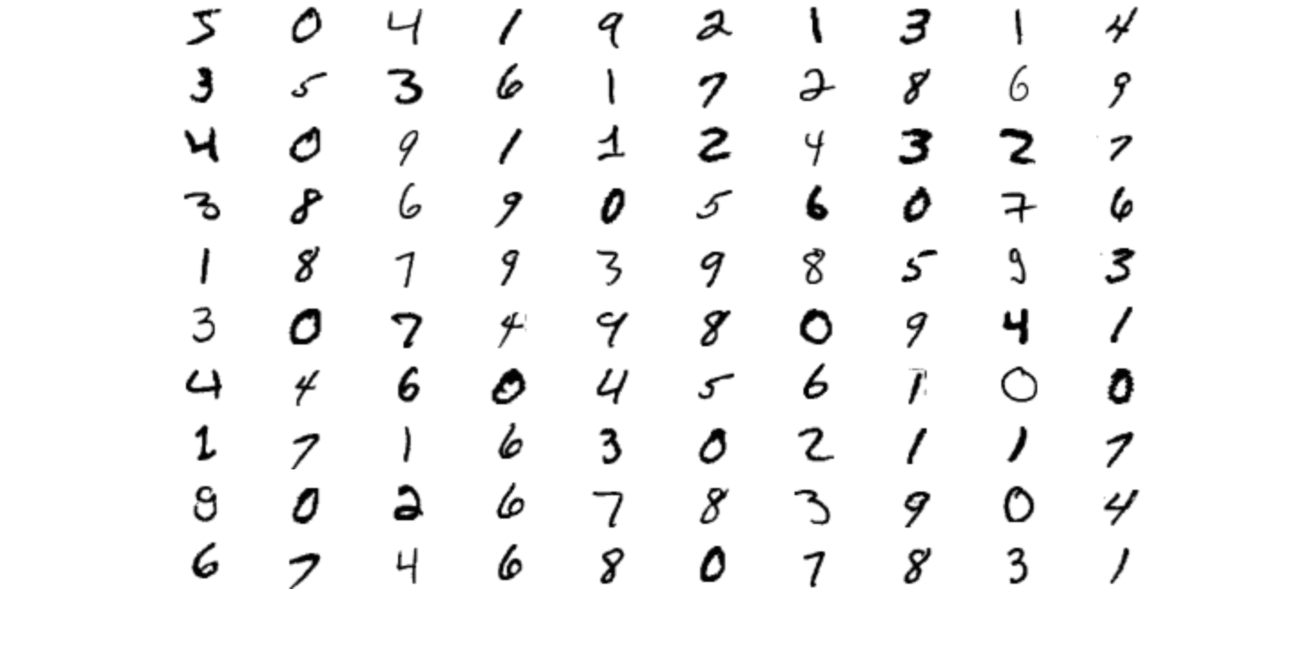
Notice that each one of the above shown digits in the original dataset is represented as a matrix of size \(28 \times 28\). For example the first one is the following
# -- print(X_train[0])
[[ 0 0 0 0 0 0 0 0 0 0 0 0 0 0 0 0 0 0 0 0 0 0 0 0 0 0 0 0]
[ 0 0 0 0 0 0 0 0 0 0 0 0 0 0 0 0 0 0 0 0 0 0 0 0 0 0 0 0]
[ 0 0 0 0 0 0 0 0 0 0 0 0 0 0 0 0 0 0 0 0 0 0 0 0 0 0 0 0]
[ 0 0 0 0 0 0 0 0 0 0 0 0 0 0 0 0 0 0 0 0 0 0 0 0 0 0 0 0]
[ 0 0 0 0 0 0 0 0 0 0 0 0 0 0 0 0 0 0 0 0 0 0 0 0 0 0 0 0]
[ 0 0 0 0 0 0 0 0 0 0 0 0 3 18 18 18 126 136 175 26 166 255 247 127 0 0 0 0]
[ 0 0 0 0 0 0 0 0 30 36 94 154 170 253 253 253 253 253 225 172 253 242 195 64 0 0 0 0]
[ 0 0 0 0 0 0 0 49 238 253 253 253 253 253 253 253 253 251 93 82 82 56 39 0 0 0 0 0]
[ 0 0 0 0 0 0 0 18 219 253 253 253 253 253 198 182 247 241 0 0 0 0 0 0 0 0 0 0]
[ 0 0 0 0 0 0 0 0 80 156 107 253 253 205 11 0 43 154 0 0 0 0 0 0 0 0 0 0]
[ 0 0 0 0 0 0 0 0 0 14 1 154 253 90 0 0 0 0 0 0 0 0 0 0 0 0 0 0]
[ 0 0 0 0 0 0 0 0 0 0 0 139 253 190 2 0 0 0 0 0 0 0 0 0 0 0 0 0]
[ 0 0 0 0 0 0 0 0 0 0 0 11 190 253 70 0 0 0 0 0 0 0 0 0 0 0 0 0]
[ 0 0 0 0 0 0 0 0 0 0 0 0 35 241 225 160 108 1 0 0 0 0 0 0 0 0 0 0]
[ 0 0 0 0 0 0 0 0 0 0 0 0 0 81 240 253 253 119 25 0 0 0 0 0 0 0 0 0]
[ 0 0 0 0 0 0 0 0 0 0 0 0 0 0 45 186 253 253 150 27 0 0 0 0 0 0 0 0]
[ 0 0 0 0 0 0 0 0 0 0 0 0 0 0 0 16 93 252 253 187 0 0 0 0 0 0 0 0]
[ 0 0 0 0 0 0 0 0 0 0 0 0 0 0 0 0 0 249 253 249 64 0 0 0 0 0 0 0]
[ 0 0 0 0 0 0 0 0 0 0 0 0 0 0 46 130 183 253 253 207 2 0 0 0 0 0 0 0]
[ 0 0 0 0 0 0 0 0 0 0 0 0 39 148 229 253 253 253 250 182 0 0 0 0 0 0 0 0]
[ 0 0 0 0 0 0 0 0 0 0 24 114 221 253 253 253 253 201 78 0 0 0 0 0 0 0 0 0]
[ 0 0 0 0 0 0 0 0 23 66 213 253 253 253 253 198 81 2 0 0 0 0 0 0 0 0 0 0]
[ 0 0 0 0 0 0 18 171 219 253 253 253 253 195 80 9 0 0 0 0 0 0 0 0 0 0 0 0]
[ 0 0 0 0 55 172 226 253 253 253 253 244 133 11 0 0 0 0 0 0 0 0 0 0 0 0 0 0]
[ 0 0 0 0 136 253 253 253 212 135 132 16 0 0 0 0 0 0 0 0 0 0 0 0 0 0 0 0]
[ 0 0 0 0 0 0 0 0 0 0 0 0 0 0 0 0 0 0 0 0 0 0 0 0 0 0 0 0]
[ 0 0 0 0 0 0 0 0 0 0 0 0 0 0 0 0 0 0 0 0 0 0 0 0 0 0 0 0]
[ 0 0 0 0 0 0 0 0 0 0 0 0 0 0 0 0 0 0 0 0 0 0 0 0 0 0 0 0]]
2.1.2 pltData()
2.1.3 pltAccuracy()
The function pltAccuracy() is use to create a plot of the accuracy of the model.
def plotAccuracy(acc_history_train, acc_history_test):
    plt.figure(figsize = (12, 8))
    plt.plot(acc_history_train, marker='o', markersize=5, label='Train')
    plt.plot(acc_history_train, marker='o', markersize=5, label='Test')
    plt.legend()
    plt.gca().xaxis.set_major_locator(plt.NullLocator())
    plt.show()
2.2 Management of Model
These two functions are instead used to save/load the model. When
using keras there are two things to take care when loading/saving a
model:
- The architecture of the model, which is represented using either the json or the yaml formats.
- The weights of the model, which are saved in a file format called HDF5.
2.2.1 save_model()
The save_model() function uses the m.to_json() method of the model
class to obtain a json representation of the model and saves it to
disk, and then the m.save_weights() method to save the weights.
def save_model(m, filename):
    model_json = m.to_json()
    with open(filename + ".json", "w") as json_file:
        json_file.write(model_json)
    # serialize weights to HDF5
    m.save_weights(filename + ".h5")
2.2.2 load_model()
The load_model() function instead does the opposite: it uses the
model_from_json() function to create a model object starting from
a json representation of the model, and the m.load_weights()
method to load the weights into the model.
def load_model(filename):
    with open(filename + ".json", "r") as json_file:
        json_model = json_file.read()
        m = model_from_json(json_model)
        # load weights into new model
        m.load_weights(filename + ".h5")
        return m
2.2.3 save_history()
2.2.4 load_history()
3 Models
To prepare our data for the training of various models we will first do the following:
- Define the number of classes in a variable called
nb_classes. - Load the data from the
mnistdataset; - Reshape the data (both test and train set) so that each image is represented as a \(768\) dimensional vector instead of a \(28 \times 28\) matrix
- Compute the one-hot-encoding for the various classes.
All of these steps are done in the following code
# number of classes, each class represents a digit
nb_classes = 10
# load data, divided in train set and test set
(X_train, t_train), (X_test, t_test) = mnist.load_data()

# Change data representation from 28 x 28 matrices to 784 dimensional
# vectors with elements in the range [0, 1].
#
# After this change X_train (as well as X_test) will be matrix with
# 6000 rows and 784 columns, where each column represents a particular
# digit.
X_train = X_train.reshape(X_train.shape[0], 784)
X_train = X_train.astype('float32')
X_train /= 255

X_test = X_test.reshape(X_test.shape[0], 784)
X_test = X_test.astype('float32')
X_test /= 255

# Computes the one-hot-encoding of the various classes
T_train = np_utils.to_categorical(t_train, nb_classes)
T_test = np_utils.to_categorical(t_test, nb_classes)
We are now ready to build various models and try out how they perform.
3.1 Softmax Regression
For our first model we will build a simple softmax regression using a single layer with \(10\) neurons and using a softmax activation function.
3.1.1 Architecture
The following code takes care of compiling the architecture of our model
model0 = Sequential()
model0.add(Dense(10, input_shape=(784,)))
model0.add(Activation('softmax'))
model0.compile(loss='categorical_crossentropy', metrics=['accuracy'], optimizer='sgd')
Visually we are constructing the following neural network
By executing the summary() method we can see the number of
parameters that we have to train.
Model: "sequential"
_________________________________________________________________
Layer (type)                 Output Shape              Param #
=================================================================
dense (Dense)                (None, 10)                7850
_________________________________________________________________
activation (Activation)      (None, 10)                0
=================================================================
Total params: 7,850
Trainable params: 7,850
Non-trainable params: 0
_________________________________________________________________
3.1.2 Training
To actually train our model we have to do the following. Notice
that as soon as we finished to train, it is crucial that we save
our model using the previously shown save_model() and
save_history() functions.
# Find the best possible function with the given data
history0 = model0.fit(X_train, T_train, batch_size=128, epochs=50, verbose=1,
                      validation_data=(X_test, T_test))

save_model(model0, 'softmax')
save_history(history0, 'softmax')
The train process then looks like this: for each epoch we see various data, such as the current value of the loss function (which as we can see it decreases over time), as well as teh current accuracy
Epoch 1/50
60000/60000 [==============================] - 1s 16us/step - loss: 0.3090 - accuracy: 0.9139 - val_loss: 0.2978 - val_accuracy: 0.9178
Epoch 2/50
60000/60000 [==============================] - 1s 16us/step - loss: 0.3082 - accuracy: 0.9144 - val_loss: 0.2972 - val_accuracy: 0.9173
Epoch 3/50
60000/60000 [==============================] - 1s 16us/step - loss: 0.3075 - accuracy: 0.9146 - val_loss: 0.2964 - val_accuracy: 0.9181
Epoch 4/50
60000/60000 [==============================] - 1s 16us/step - loss: 0.3068 - accuracy: 0.9147 - val_loss: 0.2960 - val_accuracy: 0.9173
Epoch 5/50
60000/60000 [==============================] - 1s 15us/step - loss: 0.3061 - accuracy: 0.9148 - val_loss: 0.2954 - val_accuracy: 0.9170
...
Epoch 45/50
60000/60000 [==============================] - 1s 15us/step - loss: 0.2883 - accuracy: 0.9200 - val_loss: 0.2827 - val_accuracy: 0.9207
Epoch 46/50
60000/60000 [==============================] - 1s 15us/step - loss: 0.2880 - accuracy: 0.9198 - val_loss: 0.2825 - val_accuracy: 0.9211
Epoch 47/50
60000/60000 [==============================] - 1s 15us/step - loss: 0.2877 - accuracy: 0.9199 - val_loss: 0.2823 - val_accuracy: 0.9208
Epoch 48/50
60000/60000 [==============================] - 1s 15us/step - loss: 0.2874 - accuracy: 0.9202 - val_loss: 0.2821 - val_accuracy: 0.9207
Epoch 49/50
60000/60000 [==============================] - 1s 15us/step - loss: 0.2872 - accuracy: 0.9202 - val_loss: 0.2820 - val_accuracy: 0.9210
Epoch 50/50
60000/60000 [==============================] - 1s 15us/step - loss: 0.2868 - accuracy: 0.9206 - val_loss: 0.2818 - val_accuracy: 0.9210
3.1.3 Testing
Once we have trained our data, we can construct a pandas frame from the history of training.
history0_df = pd.DataFrame(history0.history)
history0_df.head()
   val_loss  val_accuracy      loss  accuracy
0  0.297842        0.9178  0.308958  0.913900
1  0.297175        0.9173  0.308231  0.914367
2  0.296419        0.9181  0.307530  0.914567
3  0.295962        0.9173  0.306814  0.914717
4  0.295431        0.9170  0.306119  0.914783
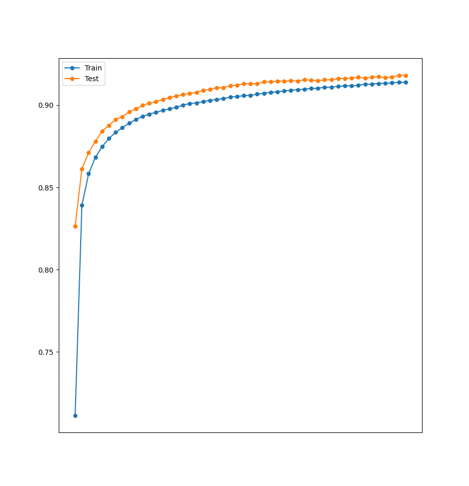
We can then use this data to show the increase in the accuracy of both the train set as well as the test set.
plotAccuracy(history0_df.accuracy, history0_df.val_accuracy)
The code above generates the following graph
Once we have our model we can also do some predictions on the test data and compute some interesting measures, such as accuracy or the f-measure with respect to each single class.
#-- do some prediction on test data
predictions_test = model0.predict_classes(X_test, verbose=0)

#-- compute accuracy of said predictions
confusion_matrix(t_test, predictions_test)
accuracy_score(t_test, predictions_test)

# -- compute for each class precision, recall and f-measure
meas = precision_recall_fscore_support(t_test, predictions_test, average=None)
for i in range(nb_classes):
    print("Class {0:d}: precision = {1:5.2f}, recall={2:5.2f}, f-measure={2:5.2f}".format(i, meas[1][i], meas[2][i], meas[3][i]))
Finally, to obtain the computed weights of the model, we can execute the following
# -- get weights
w0 = model0.layers[0].get_weights()
print(len(w0))
3.2 3-Layer NN
We will now repeat exactly every step that we did in the previous case, but this time using a 3-layer neural network.
3.2.1 Architecture
To get more than a single layers of neurons we proceed asfollows
model1 = Sequential()
model1.add(Dense(512, input_shape=(784,)))
model1.add(Activation('relu'))
model1.add(Dropout(rate=0.2))
model1.add(Dense(10))
model1.add(Activation('softmax'))
model1.compile(loss='categorical_crossentropy', metrics=['accuracy'], optimizer='adam')
3.2.2 Training
We then traing our model with the train data as follows
history1 = model1.fit(X_train, T_train, batch_size=1024, epochs=10, verbose=1,
                      validation_data=(X_test, T_test))
Once our model is trained, we save it to files for later use.
save_model(model1, 'nn3')
save_history(history1, 'nn3')
3.2.3 Testing
This time when we graph the accuracy obtained in the various epochs during training we get the following graph
history1_df = pd.DataFrame(history1)
print(history1_df.head())

plotAccuracy(history1_df.accuracy, history1_df.val_accuracy)
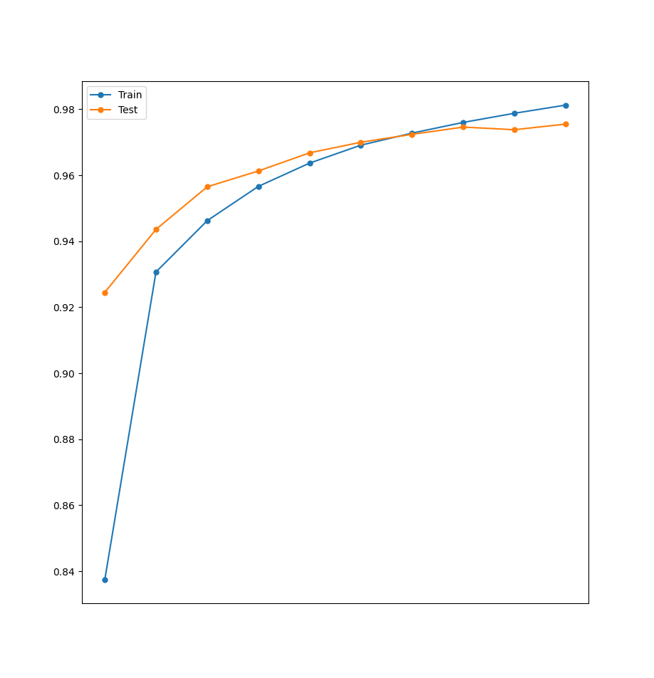
As we can see, at a certain point the accuracy of the train set keeps getting higher and higher, but the accuracy of the test set starts to decrease. This is clearly a case of overfitting.
To finish off with this model we can also do the following things using exactly the same code we showed for the previous model:
- do some predictions
- compute confusion matrix and accuracy score
- compure precision, recall and f-measure for every class
3.3 4-Layer NN
Let us now consider a 4 layer neural network.
3.3.1 Architecture
model2 = Sequential()
model2.add(Dense(512, input_shape=(784,)))
model2.add(Activation('relu'))
model2.add(Dropout(0.2))
model2.add(Dense(512))
model2.add(Activation('relu'))
model2.add(Dropout(0.2))
model2.add(Dense(10))
model2.add(Activation('softmax'))

model2.compile(loss='categorical_crossentropy', metrics=['accuracy'], optimizer='adam')
3.3.2 Training
history2 = model2.fit(X_train, T_train, batch_size=1024, epochs=10, verbose=1,
                      validation_data=(X_test, T_test))

save_model(model2, 'nn4')
save_history(history2, 'nn4')
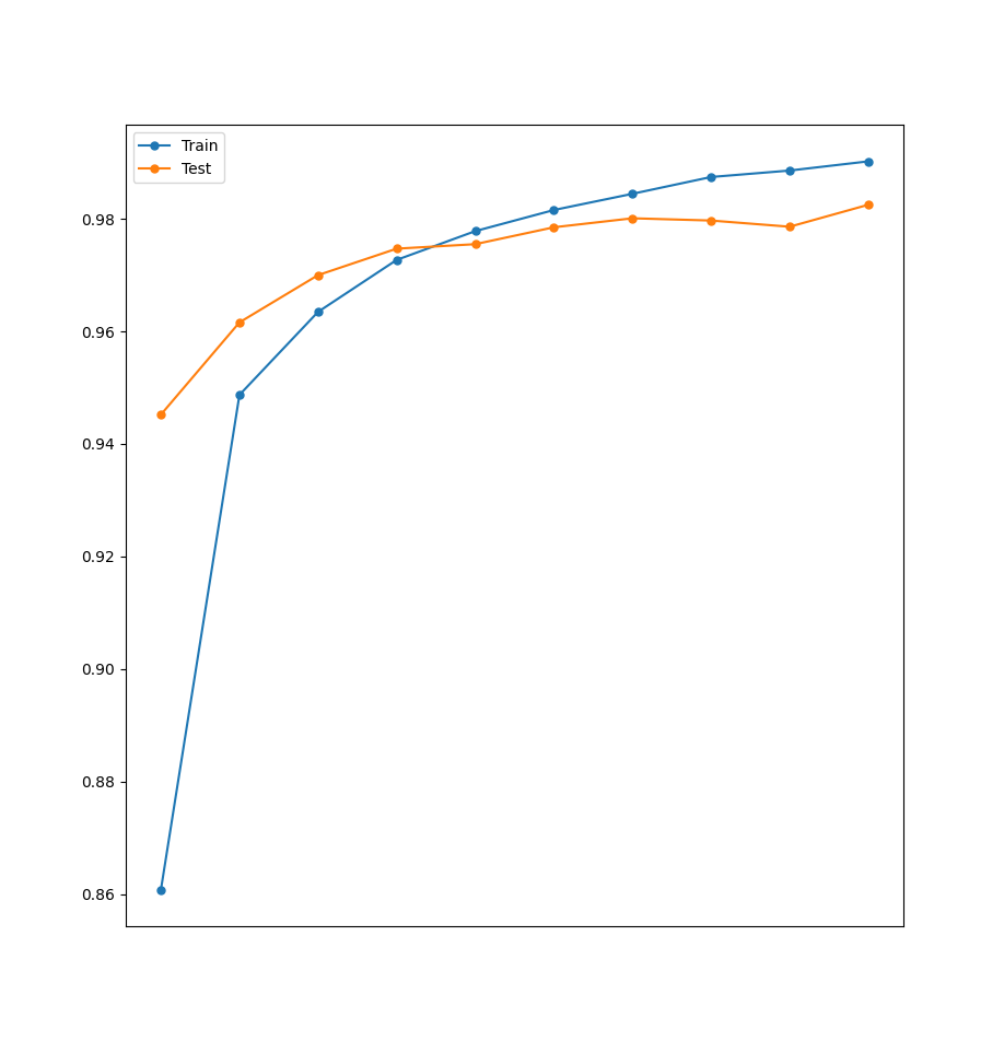
3.3.3 Testing
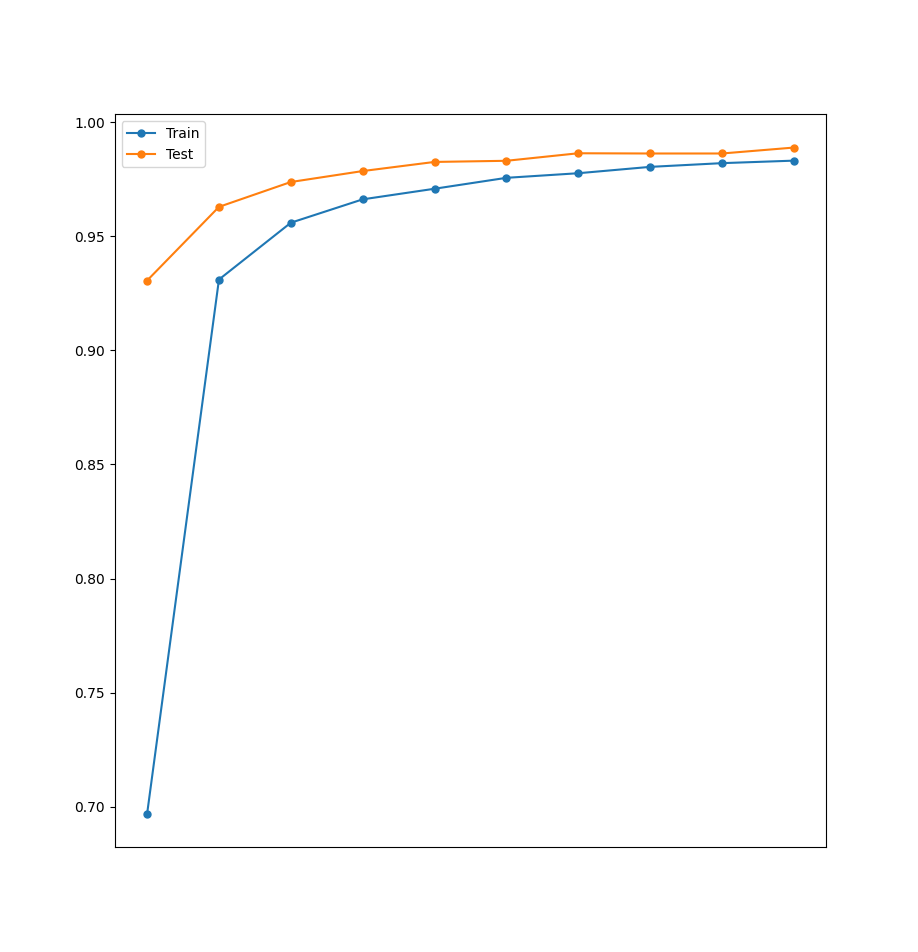
Graphing the accuracy of the training history we now get
3.4 CNN
Finally, let us consider a convoluted neural network.
3.4.1 Architecture
model3 = Sequential()
model3.add(Conv2D(30, (5, 5), input_shape=(28, 28, 1), activation='relu'))
model3.add(MaxPooling2D(pool_size=(2, 2)))
model3.add(Conv2D(15, (3, 3), activation='relu'))
model3.add(MaxPooling2D(pool_size=(2, 2)))
model3.add(Dropout(0.2))
model3.add(Flatten())
model3.add(Dense(128, activation='relu'))
model3.add(Dense(50, activation='relu'))
model3.add(Dense(10, activation='softmax'))

model3.compile(loss='categorical_crossentropy', metrics=['accuracy'], optimizer='adam')
3.4.2 Training
This time to train our model we have to change the shape of both the test data as well as the train data.
X_train_c = X_train.reshape(X_train.shape[0], 28, 28,1).astype('float32')
X_test_c = X_test.reshape(X_test.shape[0], 28, 28, 1).astype('float32')

history3 = model3.fit(X_train_c, T_train, batch_size=1024, epochs=10, verbose=1, validation_data=(X_test_c, T_test))

save_model(model3, 'cnn')
save_history(history3, 'cnn')
3.4.3 Testing
Computing our usual accuracy graph give us the following
