SICP 01B - The Substitution Model

Lecture Info

Date: [2021-03-06 sab 22:26]
Link: Lecture 1B | MIT 6.001 Structure and Interpretation, 1986
Table of contents:

In this lecture we analyzed our first model of computation: the substitution model. We then used this model to get some initial insights into how particular procedures evolve into particular processes.

1 The Substitution Model

The job of a programmer is to design processes that accomplish particular goals. This job is done by constructing spells, which are made up of procedures and expressions. These spells direct a process to accomplish the intended goal or goals. The programmer must thus understand very well the relationships between what he writes (these spells) and the behavior of the process he is attempting to control.

Suppose we want a procedure that, given two numbers, returns the sums the squares of two input numbers.

(define (sos x y)
  (+ (sq x) (sq y)))

(define (sq x)
  (* x x))

If we now execute the expression (sos 3 4) we get 25 as an answer. But how does this happen? How does this execution take place?

To answer this question we need to have a mapping which takes us from the way we write a procedure to the process it generates. We will now introduce a semi-formal mechanical model which lets us understand how, in principle, a machine could generate the process determined by a procedure. Whether or not the machine actually follows this model is completely irrelevant to us in this stage, because, like any other engineering models, the model we will introduce works in some contexts but not in some other contexts.

The model we will describe is called the substituion model, and it is the simplest model we have for understanding how procedures yield processes. This model will be accurate for a while, but eventually it will become impossible to sustain the illusion that that's the actual way the machine works. At that point we'll introduce more elaborate models.

Even though in the procedure we wrote we have different kind of expressions such as:

numbers
symbols
lambda expresisons
definitions
conditionals
combinations

to understand this model of evaluation we simply need to ask: how do we evaluate a generic combination in the substitution model? To evaluate an application the model works as follows:

First we evaluate the operator to get procedure.
Then we evalaute the operands to get the arguments.
Finally we apply the procedure to the arguments by
1. Copying the body of the procedure, substituting the arguments supplied for the formal parameters of the procedure.
2. Evaluating the resulting new body.

1.1 Example

Let us now apply mechanically an execution of the substituion model

(sos 3 4)
(+ (sq 3) (sq 4))
(+ (sq 3) (* 4 4))
(+ (sq 3) 16)
(+ (* 3 3) 16)
(+ 9 16)
25

Notice how in this model we first evaluate the procedure and then the arguments, and only then apply the procedure with the given arguments. It is entirely possible to first apply the procedure by substituting the formal parameters with the operands, and only then eveluate the operands (this order of evaluation is called the normal order evaluation).

Observation: When working with computers at any level of abstraction we can always look deeper into how something is implemented. However, to understand things, we will have to learn how to ignore details. The thing to keep in mind for understanding complex things is to understand where to not look at, and what not to compute, and what not to think.

1.2 Evaluating Conditionals

A conditional has the following form

(If <predicate> 
 <consequent>
 <alternative>)

where the is either true or false, the is the action you do in case the is true, and is the action you do otherwise, that is when the is false.

To evaluate an if expression in the substitution model the following steps are taken

First you evaluate the predicate expression.
if that yields TRUE , then you evalaute the consequent expression.
Otherwise you evaluate the alternative expression.

Let us now see this in action by first defining the following procedure, which computes the sum of two numbers using what is called Peano arithmetic.

(define (+ x y)
  (if (= x 0)
      y
      (+ (- x 1) (+ y 1))))

We can now understand how (+ 3 4) is computed using the above model

(+ 3 4)
(if (= 3 0) 4 (+ (- 3 1) (+ 4 1)))
(+ (- 3 1) (+ 4 1))
(+ 2 5)
(if (= 2 0) 5 (+ (- 2 1) (+ 5 1)))
(+ (- 2 1) (+ 5 1))
(+ 1 6)
(if (= 1 0) 6 (+ (- 1 1) (+ 6 1)))
(+ (- 1 1) (+ 6 1))
(+ 0 7)
(if (= 0 0) 7 (+ (- 0 1) (+ 7 1)))
7

Observation: It's important to get the name of things or parts of expression, because every sorcerer will tell you that to have power over a spirit, you have to name them.

1.3 Shapes of Processes

We will now see start to understand how particular programs evolve into particular processes, and how to shape our programs to get specific shapes in the process they generate.

Observation: The key of being a creative photographer is being able to understand what you will get on camera before actually pushing the button. Can I imagine in my mind the resulting image very precisely as a consequence of the particular framing and of various other things?

We will now see two different procedures which represent two different ways of adding whole numbers. These two programs will be almost identical, but they will generate two different processes.

1.3.1 (Linear) Iteration

First we consider the sum of x and y to be the sum of the decrement of the first and the increment of the second.

(define (+ x y)
  (if (= x 0)
      y
      (+ (-1+ x) (1+ y))))

Consider now an execution of procedure

(+ 3 4)
(+ 2 5)
(+ 1 6)
(+ 0 7)
7

This algorithm takes time \(O(x)\), that is proportional to \(x\), while the amount of space is costant \(O(1)\). Such a process is called an (linear) iteration.

1.3.2 (Linear) Recursion

Now we consider the sum of x and y as the increment of the sum of the decrement of the first with the second.

(define (+ x y)
  y
  (1+ (+ (-1+ x) y)))

Consider now an executing on this second procedure.

(+ 3 4)
(1+ (+ 2 4))
(1+ (1+ (+ 1 4)))
(1+ (1+ (1+ (+ 0 4))))
(1+ (1+ (1+ 4)))
(1+ (1+ 5))
(1+ 6)
7

The second algorithm has a time complexity that is also \(O(x)\), while the space complexity is \(O(x)\). This kind of process is called a (linear) recursion.

1.3.3 Iteration vs Recursion

Notice that the first process was sort-of "straight", while the second one gets "bigger" and then "smaller".

Notice also that both of the procedures were defined in a recursive manner. Yet, they lead to different shapes processes. Thus, it is not always the case that a recursive definition leads to a recursive process.

Another difference between iteration and recursion is: how much stuff is under the table? That is, suppose I stop the computation at some point, how much memory in this would a state require? In the example of iteration, I would only need to know the values of the parameters of the procedure, since an iteration has all of its state in explicit variables. A recursion is not quite the same, because, in a recursion I would need to also keep in mind what was saved in the state of the machine.

2 Examples

Let us finish this lecture by presenting two different problems.

2.1 Fibonacci

Consider the sequence of Fibonacci numbers

\[1 \,\,\, 1 \,\,\, 2 \,\,\, 3 \,\,\, 5 \,\,\, 8 \,\,\, 13 \,\,\, 21 \,\,\, 34 \,\,\, 55\]

defined in the following way

\[F_n = \begin{cases} 1 &,\,\, n=1, 2 \\ F_{n-1} + F_{n-2} &,\,\, n > 2 \\ \end{cases}\]

These numbers can be computed with the following procedure

(define (fib n)
  (if (< n 2)
      n
      (+ (fib (- n 1))
         (fib (- n 2))))))

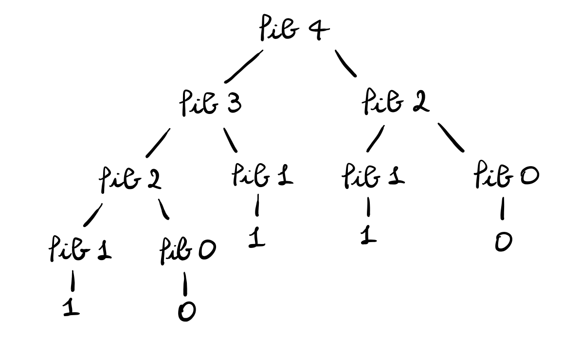
This is an extreme bad way of computing fib since we have to many re-computation. Indeed, if we assume that we're doing everything sequentially, then this process has a time complexity of \(O(Fib n)\). In terms of space instead, this procedure takes \(O(n)\).

To give an intuition behind these results, consider the tree graph obtained by computing (fib 4) and observing every recursive call being made.

Observation: Programming is hard because you have to write very general rule that take care of all the possible inputs.

2.2 Towers of Hanoi

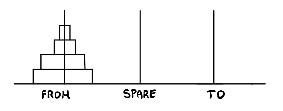
Consider the famous problem of the Towers of Hanoi: you have a rod on which there is an n-layered tower made up of disks of various size.

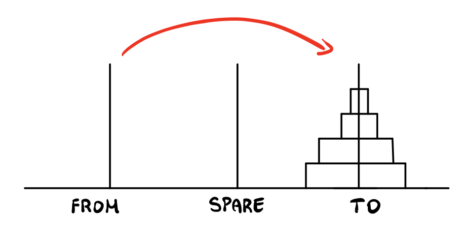
Your objective is to move such tower to another rod such that, at any point in time, you cannot place a larger disk on top of a smaller one.

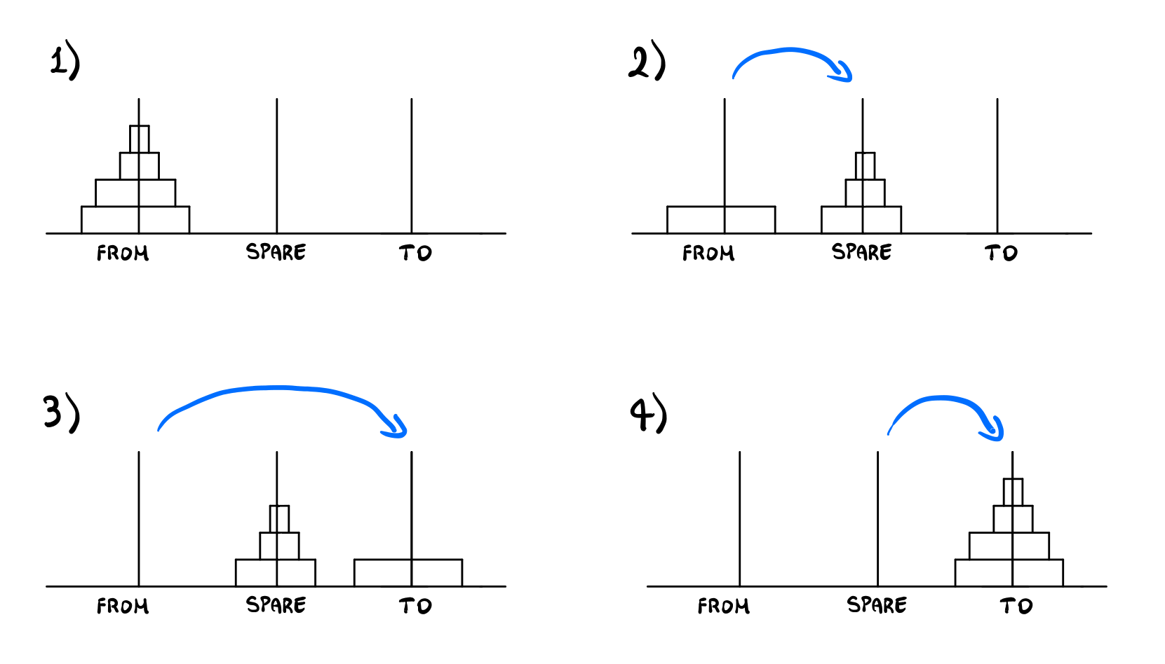
To solve this problem the idea is to construct a recursive proces by wishful thinking . Consider for example an instance of the problem where \(n=4\), and assume, by wishful thinking, that we can solve the problem for the case where \(n=3\). Then we can do the following steps

Now you might be thinking: okay, but now I have to learn how to move a tower of \(3\) disks, so have I solved anything?. And yes, that is true, we still have to learn how to move a tower of \(3\) disks. Yet, if we remember our original problem was how to move a tower of \(4\) disks. That is, now our problem is simpler, because it has less disks. And since our reasoning does not depend on the number of disks, we can iterate again and again, until we reach a tower of \(1\) disk, which can be moved to any rod without problems.

The procedure which implements this recursive strategy is the following

(define (move N FROM TO SPARE)
  (cond ((= N 1) "DONE")
        (else
         (move (- N 1) FROM SPARE TO)
         (PRINT-MOVE FROM TO)
         (move (- N 1) SPARE TO FROM))))

Finally, consider the move generated by the algorithm for a \(4\) disks instance.

(move 4 1 2 3)
(move 3 1 3 2)
(move 2 1 2 3)
(move 1 1 3 2)
(move 0 1 2 3)
DONE
(PRINT-MOVE 1 3)
...

Can you write an iterative algorithm rather than a recursive algorithm that solve the same problem?